Backpropagation

Backpropagation, short for Backward Propagation of Errors, is the core algorithm used to train neural networks. It uses the Chain Rule to calculate how much each weight and bias contributed to the total error, allowing us to update them and improve the model's accuracy.

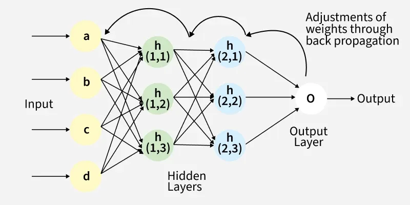
The Intuition: Why Backwards?

Think of the Forward Pass as "making a prediction" and the Backward Pass as "distributing the blame." When the network makes a mistake, we calculate the error at the output. To fix it, we need to know how each neuron in the previous layers influenced that error. By moving backward, we can efficiently "propagate" the error signal using the chain rule, calculating gradients layer by layer without redundant computations.

Steps of Backpropagation

After the forward pass through the network and the calculation of the loss using a cost function, backpropagation proceeds with the following steps:

1. Gradients Calculation: For each learnable parameter (weights and biases) in the network, we compute the gradient of the loss function with respect to that parameter. This is done using the Chain Rule of calculus. (See Gradient Descent for how we use these gradients to actually improve the model.)

2. Weight and Bias Updates: Once the gradients are computed, we update the weights and biases using an optimization algorithm, typically Gradient Descent. The parameters are adjusted in the direction that reduces the loss, scaled by a learning rate that controls the step size of the updates. The update rule for a weight $( w )$ is given by:

   $$w := w - \eta \frac{\partial L}{\partial w}$$

   Where:

   • $\eta$ is the learning rate
   • $\frac{\partial L}{\partial w}$ is the gradient of the loss with respect to the weight $w$

3. Iteration: Steps 1 and 2 are repeated for multiple epochs (iterations) until the network converges to a satisfactory level of accuracy.

Gradients

Situation: We consider a multi-class classification problem with a neural network that has multiple layers. The hidden layers use the Sigmoid activation function, and the output layer uses the Softmax activation function. The cost function used is Cross-Entropy Loss.

Output Layer

Our CE loss defined as $C = - \sum_{i=1}^{n} y_i \log(\hat{y}_i)$ where $n = s[L]$ is the number of classes, and $\hat{y}_i = a_i^{(L)}$ is the output of the Softmax function for class $i$ (neuron $i$ in the output layer).

The gradient of the loss w.r.t the $\hat{y}_i$ is given by:

$$\boxed{\frac{\partial C}{\partial \hat{y}_i} = - \frac{y_i}{\hat{y}_i}}$$

note

That gradient only depends on the $\hat{y}_i$ and any other term in the summation where $i \neq j$ is treated as a constant.

The gradient of the $\hat{y}_i$ w.r.t the input $z_i$ of the Softmax function is:

$$\frac{\partial \hat{y}_i}{\partial z_k} = \frac{\delta_{ik} e^{z_i} S - e^{z_i} e^{z_i}} {S^2}$$

note

Here $\hat{y}_i$ does depend on all $z_k$ because of the denominator $S = \sum_{k} \exp(z_k)$ from the Softmax function.

Simplifying this, we get:

$$\frac{\partial \hat{y}_i}{\partial z_k} = \hat{y}_i (\delta_{ik} - \hat{y}_k)$$

Thus, for $z_i$:

$$\boxed{\frac{\partial \hat{y}_i}{\partial z_i} = \hat{y}_i (1 - \hat{y}_i)}$$

where:

• $\delta_{ik}$ is the Kronecker delta, which is 1 if $i = j$ and 0 otherwise.
• $S = \sum_{k} \exp(z_k)$

Then, using the chain rule, the gradient of the loss w.r.t the input $z_i$ of the Softmax function is:

$$\frac{\partial C}{\partial z_i} = \sum_{n} \frac{\partial C}{\partial \hat{y}_n} \frac{\partial \hat{y}_n}{\partial z_i}$$ $$= \sum_{n} \left( - \frac{y_n}{\hat{y}_n} \right) \hat{y}_n (\delta_{ni} - \hat{y}_i)$$ $$= \sum_{n} \left( - y_n (\delta_{ni} - \hat{y}_i) \right)$$ $$= -y_i + \sum_{n} y_n \hat{y}_i$$

And since $\sum_{n} y_n = 1$ for one-hot encoded labels, we have:

$$\boxed{\frac{\partial C}{\partial z_i} = \hat{y}_i - y_i = \Delta_i}$$

We have $z_i^{l} = W_i^{l} A_{prev} + b_i$ where $W_i^{l}$ is the weights of current layer in neuron $i$, $A_{prev}$ is the activations from the previous layer, and $b_i$ is the bias for neuron $i$.

Thus, the gradients for the weights and biases in the output layer are:

$$\frac{\partial C}{\partial W_i} = \frac{\partial C}{\partial z_i} \cdot A_{prev}^T$$ $$\boxed{\frac{\partial C}{\partial W_i} = (\hat{y}_i - y_i) \cdot A_{prev}^T}$$ $$\boxed{\frac{\partial C}{\partial b_i} = \hat{y}_i - y_i}$$

Summary: Vectorized Gradients

To implement backpropagation efficiently for a batch of $m$ examples, we use the following vectorized equations. These avoid explicit loops over individual neurons or examples.

Vectorized Equations

For any layer $l$:

1. Error Signal ($\Delta$): $\Delta^{(l)} = \frac{\partial C}{\partial Z^{(l)}}$
2. Weight Gradient ($dW$): $dW^{(l)} = \frac{1}{m} \Delta^{(l)} (A^{(l-1)})^T$
3. Bias Gradient ($db$): $db^{(l)} = \frac{1}{m} \sum_{i=1}^{m} \Delta^{(l)}_i$
4. Activation Gradient ($dA_{prev}$): $dA^{(l-1)} = (W^{(l)})^T \Delta^{(l)}$

Python Implementation

backpropagation.py

import numpy as np
from typing import List, Callable
from activation_functions import Activation_Functions
from cost_functions import Cost_Functions

np.random.seed(42)

class NN:
    def __init__(self, s: List[int]):
        '''
        s: List of layer sizes, where s[0] is the input layer size, s[1] is the first hidden layer size, ..., s[L] is the output layer size
        '''
        self.s = s
        self.L = len(s) - 1 
        self.weights = [np.random.randn(s[l], s[l-1]) * 0.01 for l in range(1, self.L + 1)]
        self.biases = [np.zeros((s[l], 1)) for l in range(1, self.L + 1)]
        self.f = Activation_Functions.sigmoid
        self.f_output = Activation_Functions.softmax
        self.cost = Cost_Functions.ce
        self.cost_grad = Cost_Functions.ce_grad

    def forward_pass(self, X: np.ndarray) -> (np.ndarray, List[tuple]):
        # ...
        pass

    def compute_cost(self, AL: np.ndarray, Y: np.ndarray) -> float:
        # ...
        pass
    
    def backpropagation(self, AL: np.ndarray, Y: np.ndarray, cache: List[tuple]) -> dict:
        '''
        AL: Output of the network from forward pass
        Y: True labels (one-hot encoded)
        cache: List of tuples containing (A_prev, W, b, Z) for each layer from forward pass

        Returns:
            grads: Dictionary containing gradients for weights and biases e.g., {'dW1': ..., 'db1': ..., 'dW2': ..., 'db2': ..., ...}
        '''
        grads = {}
        m = Y.shape[1] # number of examples

        # ---- 1. Output Layer ----
        Delta_L = AL - Y # (s[L], m)
        A_prev, W_L, b_L, Z_L = cache[-1]

        # grads
        grads[f'dW{self.L}'] = (1/m) * np.dot(Delta_L, A_prev.T)
        grads[f'db{self.L}'] = (1/m) * np.sum(Delta_L, axis=1, keepdims=True)

        # ---- 2. Hidden Layers ----
        Delta_next = Delta_L
        dA_prev = np.dot(W_L.T, Delta_next)

        for l in reversed(range(self.L - 1)):
            A_prev, W_l, b_l, Z_l = cache[l]

            Delta_l = dA_prev * Activation_Functions.sigmoid_derivative(Z_l)

            # grads
            grads[f'dW{l+1}'] = (1/m) * np.dot(Delta_l, A_prev.T)
            grads[f'db{l+1}'] = (1/m) * np.sum(Delta_l, axis=1, keepdims=True)

            dA_prev = np.dot(W_l.T, Delta_l)
        
        return grads
    
    def update_parameters(self, grads: dict, learning_rate: float = 0.001):
        for l in range(self.L):
            self.weights[l] -= learning_rate * grads[f'dW{l+1}']
            self.biases[l] -= learning_rate * grads[f'db{l+1}']

Remember

• $L$: Index of last layer (output layer).
• $dW[l]$: Gradient of weights for layer with index $l$.
• $cache[l]$: Cached values for layer with index $l-1$.
• $weights[l]$: Weights for layer with index $l-1$.