Forward Pass

In a neural network, the Forward Pass is the initial step where input data is passed through the network to generate an output. This process involves computing the weighted sum of inputs, adding biases, and applying activation functions at each neuron in the network.

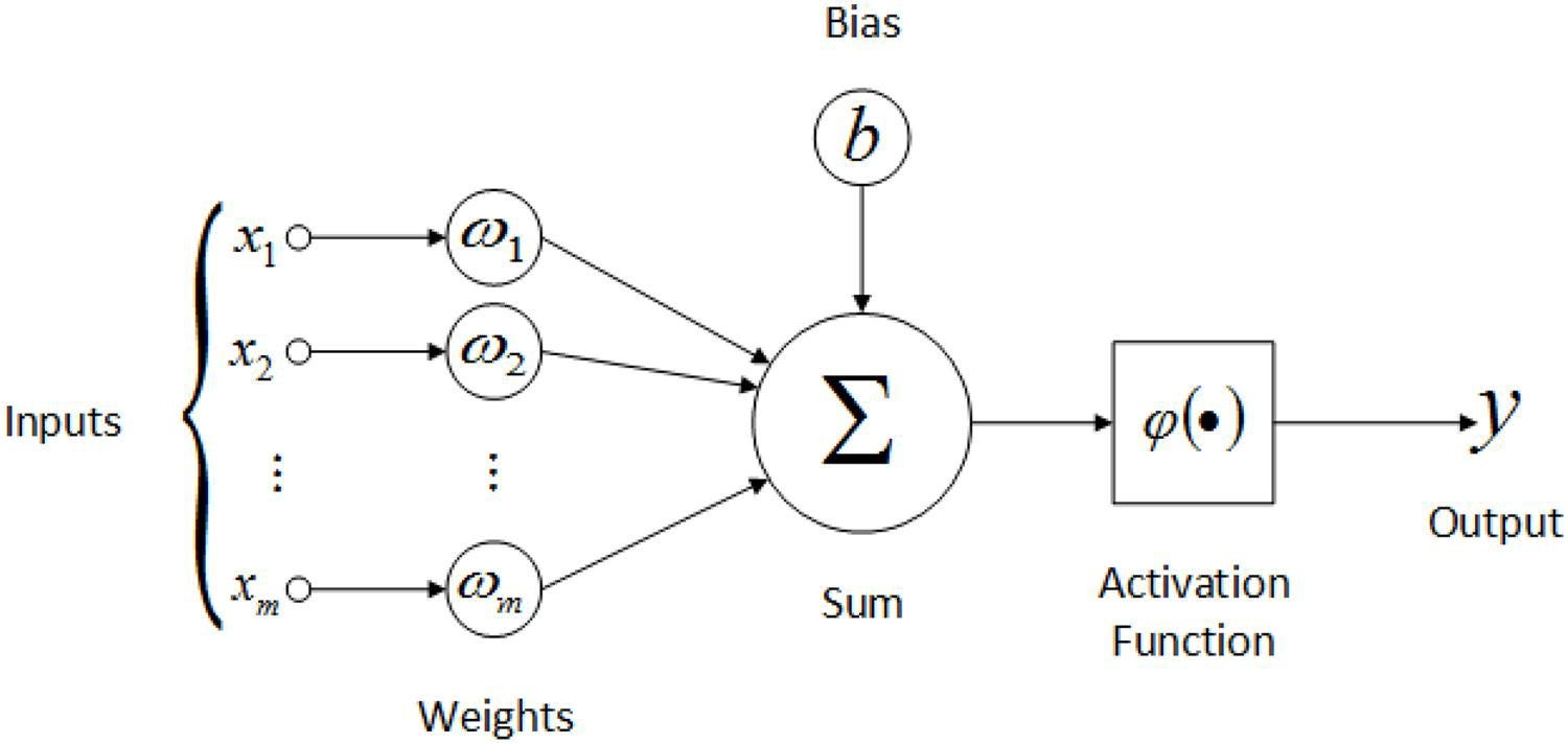
Steps in Forward Pass

1. Input Layer: The input data is fed into the network through the input layer. Each feature of the input data corresponds to a neuron in this layer. So the number of neurons in the input layer equals the number of features in the input data.

2. Hidden Layers: The data is then passed to one or more hidden layers. Each neuron in a hidden layer performs the following operations:

   • Computes the weighted sum of its inputs.
   • Adds a bias term.
   • Applies an activation function to introduce non-linearity. (See Activation Functions for more details.)

   Mathematically, for a single neuron ( j ) in layer ( l ):

   $$z_j^{(l)} = \sum_{i} w_{ij}^{(l)} a_i^{(l-1)} + b_j^{(l)}$$ $$a_j^{(l)} = f(z_j^{(l)})$$

Vectorization: From Neurons to Matrices

In practice, we don't compute the forward pass neuron-by-neuron. Instead, we use matrix operations to process entire layers and multiple training examples (batches) simultaneously. This is known as vectorization and is significantly faster on modern hardware (CPUs/GPUs).

1. Layer-wise Vectorization

We combine all weights for layer $l$ into a weight matrix $W^{(l)}$ and all biases into a vector $b^{(l)}$. The linear transformation for the entire layer becomes:

$$Z^{(l)} = W^{(l)} A^{(l-1)} + b^{(l)}$$

2. Batch Vectorization

When processing $m$ training examples at once, $A^{(l-1)}$ becomes a matrix of shape $(n_{l-1}, m)$. The resulting $Z^{(l)}$ and $A^{(l)}$ will have shape $(n_l, m)$, where each column represents one example in the batch.

Notation Guide

Indices & Dimensions

• $l$: Current layer index ($0$ = input, $L$ = output).
• $m$: Number of training examples in the batch.
• $n_l$: Number of neurons in layer $l$.

Variables & Matrices

• $X$: Input matrix. Shape: $(n_0, m)$.
• $W^{(l)}$: Weight matrix for layer $l$. Shape: $(n_l, n_{l-1})$.
• $b^{(l)}$: Bias vector for layer $l$. Shape: $(n_l, 1)$.
• $Z^{(l)}$: Linear output (pre-activation). Shape: $(n_l, m)$.
• $A^{(l)}$: Activation output (post-activation). Shape: $(n_l, m)$.

Python Implementation

neural_netwrok.py

import numpy as np
from typing import List, Callable
from activation_functions import Activation_Functions
from cost_functions import Cost_Functions

np.random.seed(42)

class NN:
    def __init__(self, s: List[int]):
        '''
        s: List of layer sizes, where s[0] is the input layer size, s[1] is the first hidden layer size, ..., s[L] is the output layer size
        '''
        self.s = s
        self.L = len(s) - 1 
        self.weights = [np.random.randn(s[l], s[l-1]) * 0.01 for l in range(1, self.L + 1)]
        self.biases = [np.zeros((s[l], 1)) for l in range(1, self.L + 1)]
        self.f = Activation_Functions.sigmoid
        self.f_output = Activation_Functions.softmax
        self.cost = Cost_Functions.ce
        self.cost_grad = Cost_Functions.ce_grad

    def forward_pass(self, X: np.ndarray) -> (np.ndarray, List[tuple]):
        '''
        X: Input data of shape (n, m)
        '''
        cache = [] # Stores (A_prev, W, b, Z) for each layer to be used during Backpropagation
        A = X

        for l in range(self.L):
            A_prev = A

            W = self.weights[l]
            b = self.biases[l]
            # Linear Step
            Z = np.dot(W, A_prev) + b
            # Activation Step
            if l == self.L - 1:
                A = self.f_output(Z)
            else:
                A = self.f(Z)
            
            cache.append((A_prev, W, b, Z))

        return A, cache

    def compute_cost(self, AL: np.ndarray, Y: np.ndarray) -> float:
        cost = self.cost(Y, AL)
        return cost