MAGIC'24 USENIX

Prerequisites

$(M, \color{blue}K)$

To deconstruct this paper effectively, we will need three foundations:

• Provenance Graphs that you can check here
• Graph Attention Networks (GAT) you can check them here
• Graph Masked Autoencoders (GMAE) available also here

To have an idea about what datasets being used and the difference between them:

• Streamspot that you can check here
• DARPA TC E3 and CDM v.18 Schema that you can check here

Problem State & Motivation

In the introduction, the authors identified three major limitations of existing approaches (Supervised, Statistic-based and DL-based):

Supervised

The authors highlighted two critical weaknesses of using Supervised Learning for this kind of security:

• Lack-Of-Data (LOD): Real APT attacks are rare, so there are not enough labeled example to train supervised models on.
• Vulnerability to New Types: Supervised models are essentially pattern-matchers. If an attack doesn't match the specific patterns the model was trained on (like a "zero-day" or a new variant), the model is blind to it.

This puts us in a bind: We can't train the model on attacks because we don't have enough data, and even if we did, it wouldn't catch the next new attack.

The Solution: Flipping the Script

Since we can't effectively model the attacks, the authors proposed to model benign (normal) behavior instead. MAGIC learns to be an expert on what "healthy" system activity looks like. Anything that deviates from that standard is flagged as suspicious. This approach is formally called Anomaly Detection.

Statistic-based

According to the paper, Statistic-based approaches (which use things like rarity or anomaly scores). have three main weaknesses:

• Rarity $\neq$ Malice: They assume that if a system entity (like a process or file) is "rare," it is likely malicious. The authors argue this is often false; many benign system behaviors are rare but safe.
• Shallow Understanding: These methods perform shallow feature extraction. They look at surface-level numbers but fail to understand the deep semantics or the story behind the data.
• High False Positives: Because they flag things based on simple rarity without understanding the context, they tend to raise too many false alarms (False Positives).

The Solution: Deep Graph Representation Learning

Graph Representation Module converts system entities into embeddings which captures complex, multi-dimensional information about what the entity is and how it behaves. It also captures contextual information to understand the full story.

DL-based

While DL-based methods are powerful, the authors point out a major practical flaw that often prevents them from being used in the real world. The primary issues are related to effeciency and resources.

• Computational Overhead: Existing Graph-based and Sequence-based DL methods are extremely "heavy". In a real entreprise, hundreds of gigabytes of logs are produced daily. Processing such a large volume with standard DL models is often too slow to be practical. (For example ATLAS takes about 1 hour to train on $676Mb$ of logs, and ShadeWatcher takes 1 day to train on DARPA dataset even with a GPU.)
• Memory Consumption: Some Graph Auto-Encoder approaches suffer from "Explosive Memory Overhead" as the graph gets larger (scalling issues).

The Solution: Effeciency Through Masking

MAGIC addresses these resource problems directly with it Masked Graph Auto-Encoder (MGAE) architecture.

MAGIC Architecture

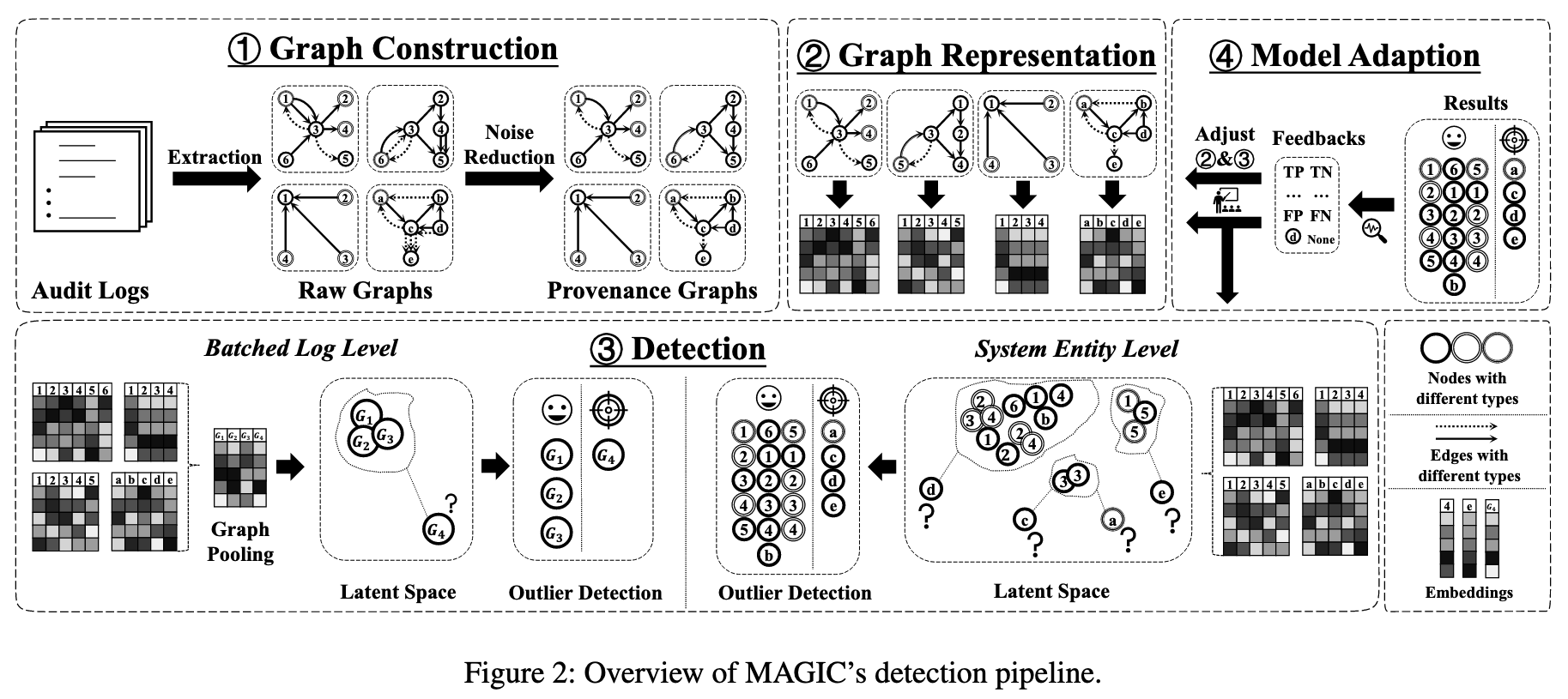
Now that we know MAGIC's strategy is to learn benign behavior efficiently, we need to understand its architecture. The Figure 2 (below) provides the roadmap for this process.

1. Graph Construction

Turning raw logs into a structured graph

Real-world audit logs are just massive list of text lines. Before the AI can learn anything, MAGIC needs to turn these lists into a clean Provenance Graph.

According to §4.1 (Provenance Graph Construction), the process is divided into three distinct steps:

1. Log Parsing: Extracting entities and interactions from the raw text logs to build a "prototype" graph. After extraction, we normalize the different ways of representing the same entity or interaction. For instance, a raw log might show sys_open, sys_openat or sys_creat, but we normalize them all under a single abstract edge type OPEN. The result of this step is a Provenance Graph where nodes are entities defined with attributes (or ID) and types, along with edges defined by source, destination and edge type.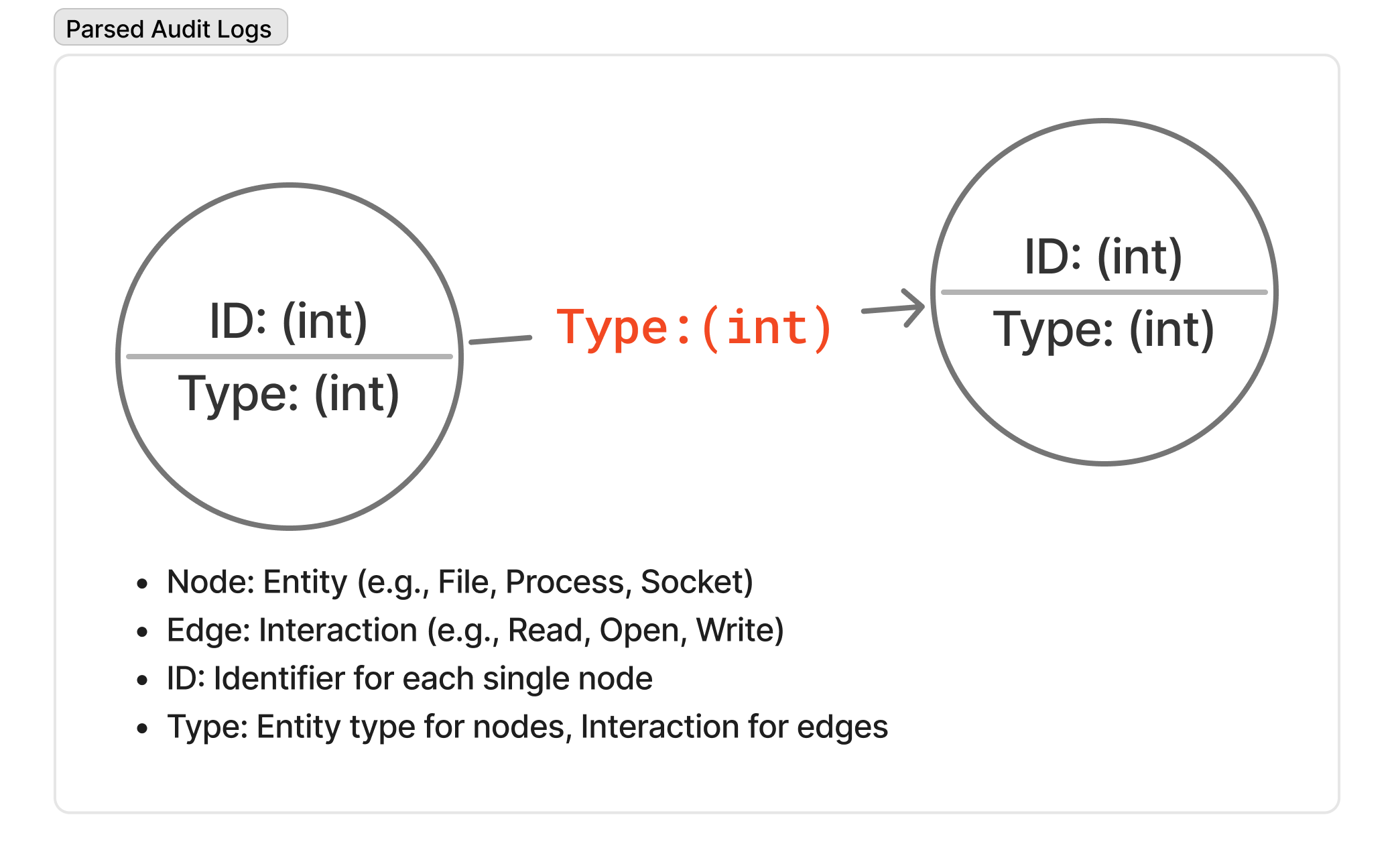

   

   Illustrated Examples

   Check examples in Streamspot Dataset and DARPA TC E3 Dataset.

2. Initial Embeddings: Converting the labels (Type IDs) of these nodes and edges into feature vectors. According to §4.1 (Initial Embeddings), this step transforms the labels into a fixed-size feature vector of dimension $d$. The paper describes the Lookup Embedding approach, which is a simple yet effective way to convert labels into embeddings. They mentions that node/edge labels are determined by the data source. Therefore, the lookup embedding is transductive and do not need to learn embeddings for unseen labels.

   From the Implementation Source Code, we can see that OneHot Encoding is used to convert the labels into feature vectors.

   new_g.ndata['attr'] = F.one_hot(g.ndata['type'].view(-1), num_classes=node_feat_dim).float()
   new_g.edata['attr'] = F.one_hot(g.edata['type'].view(-1), num_classes=edge_feat_dim).float()

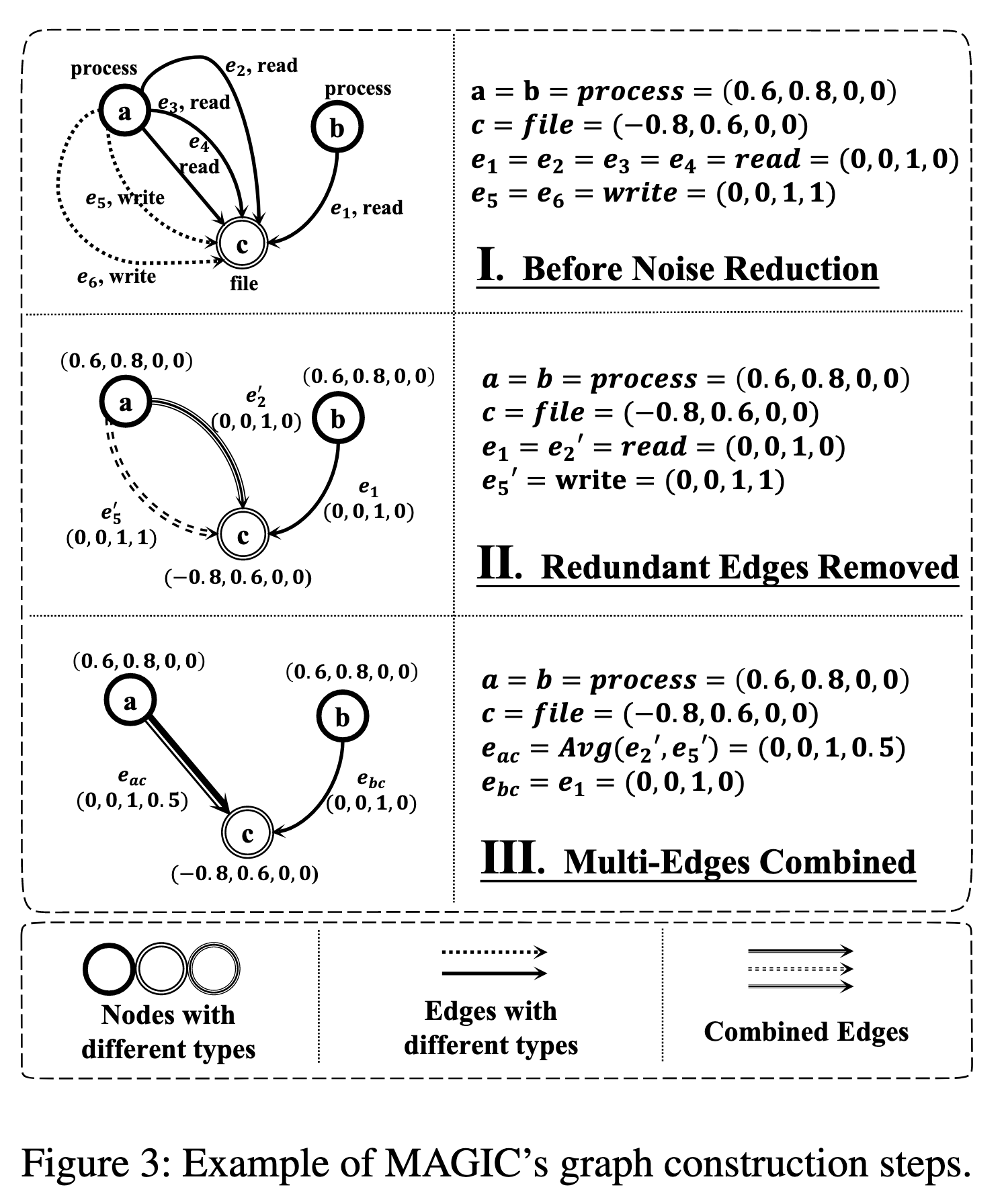
3. Noise Reduction: In real system logs, a process might read a file 1,000 times in a row. If we kept every single one of those as a separate edge, the graph would be gigantic and slow to process. According to §4.1 (Noise Reduction), MAGIC simplifies this "Multi-Graph" into a "Simple Graph" using two rules :

   • Duplicate Removal: If there are multiple edges of the same type (e.g., 50 READ edges) between two nodes, it keeps just one.
   • Type Combination: If there are edges of different types (e.g., one READ and one WRITE) between two nodes, it combines them into a single edge.

   

2. Graph Representation

The "brain" MGAE that learns the embeddings

According to §4.2 (Graph Representation) and Figure 4 of the paper, the Graph Representation Module is divided into three distinct phases:

1. Feature Masking (4.2.1): To make the model learn on its own (self-supervised), MAGIC plays a game of "fill-in-the-blank." It randomly selects a percentage of nodes and replaces their initial features (vectors) with a generic MASK token. This forces the model to guess what the missing node is by looking at its surroundings. Let $\tilde{N}$ be the set of masked nodes.

   $$emb_{n} = \begin{cases} x_{n}, & n \notin \tilde{N} \\ x_{mask}, & n \in \tilde{N} \end{cases}$$
   Detection

   During detection we do not mask any nodes.

2. Graph Encoder (4.2.2): If we look at our provenance graph, we can see that "Process A vs. Process B" with the same type "Process" have the same Initial Embeddings. The goal of the encoder is to update these vectors so they look different based on who they interact with. MAGIC uses a Graph Attention Network (GAT) to achieve this (you can learn about GATs here). In brief, GATs are a type of neural network that can process graph data by using attention mechanisms to weight the importance of different nodes in the graph. For each node, it calculates an attention score based on the node's features and the features of its neighbors. The attention score is then used to update the node's features, making them more representative of the graph's structure. Before the Encoder, a node can only say "I am a Process", but after the encoder, it can say "I am a Process that did X with Y..".

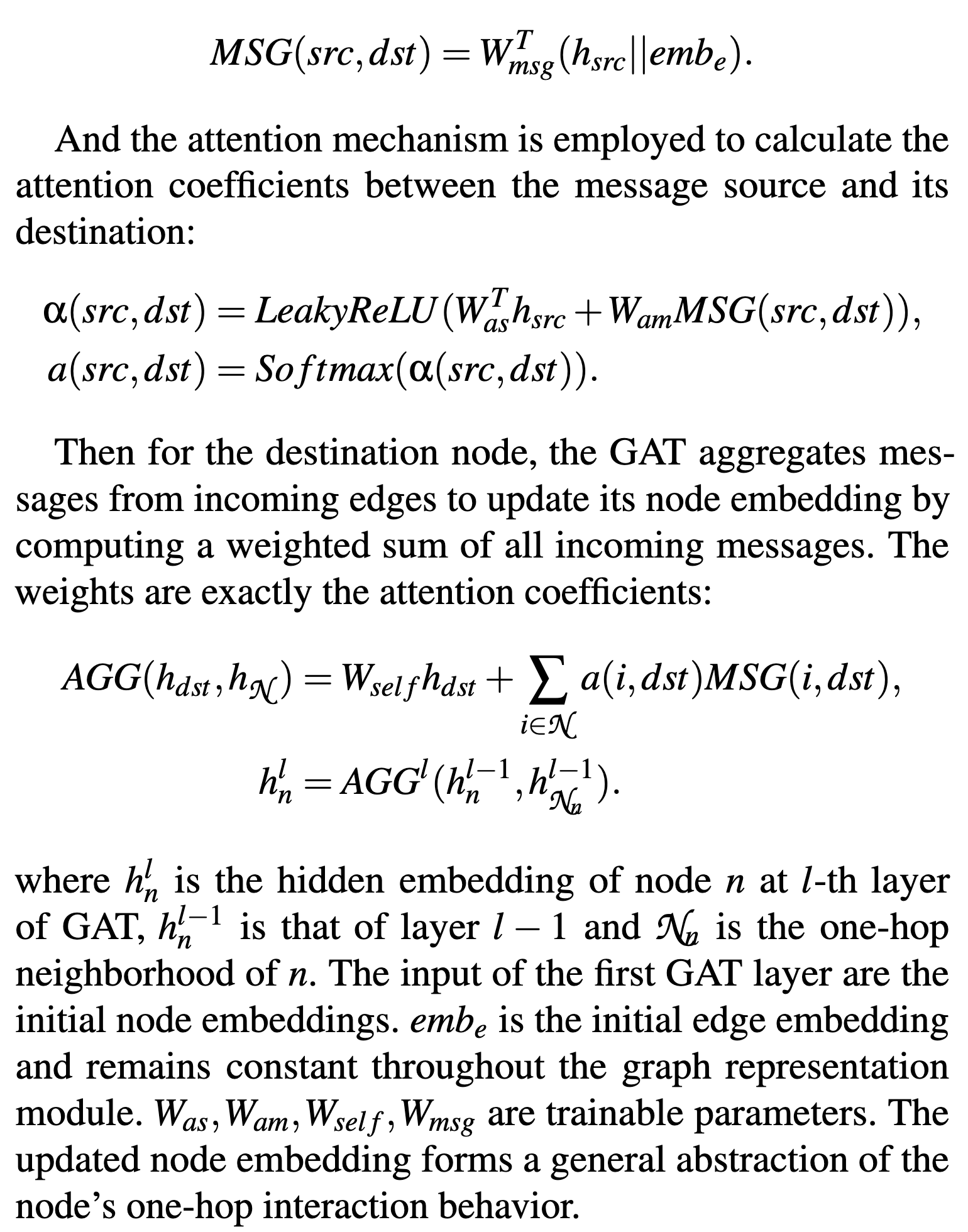
   MAGIC's encoder didn't implement the exact original GAT Message Passing and Aggregation steps. Instead, it modified the original GAT to include the edge features.

   The math behind from the paper

   

   GATConv

   class GATConv(nn.Module):
       def __init__(self,
                   in_dim,
                   e_dim,
                   out_dim,
                   n_heads,
                   feat_drop=0.0,
                   attn_drop=0.0,
                   negative_slope=0.2,
                   residual=False,
                   activation=None,
                   allow_zero_in_degree=False,
                   bias=True,
                   norm=None,
                   concat_out=True):
           super(GATConv, self).__init__()

3. Graph Decoder (4.2.3)

3. Detection

The "judge" that spots the outliers

Reference

• Magic'24 USENIX Paper